Marching Waves
My signature art style and how it’s made.
The Style
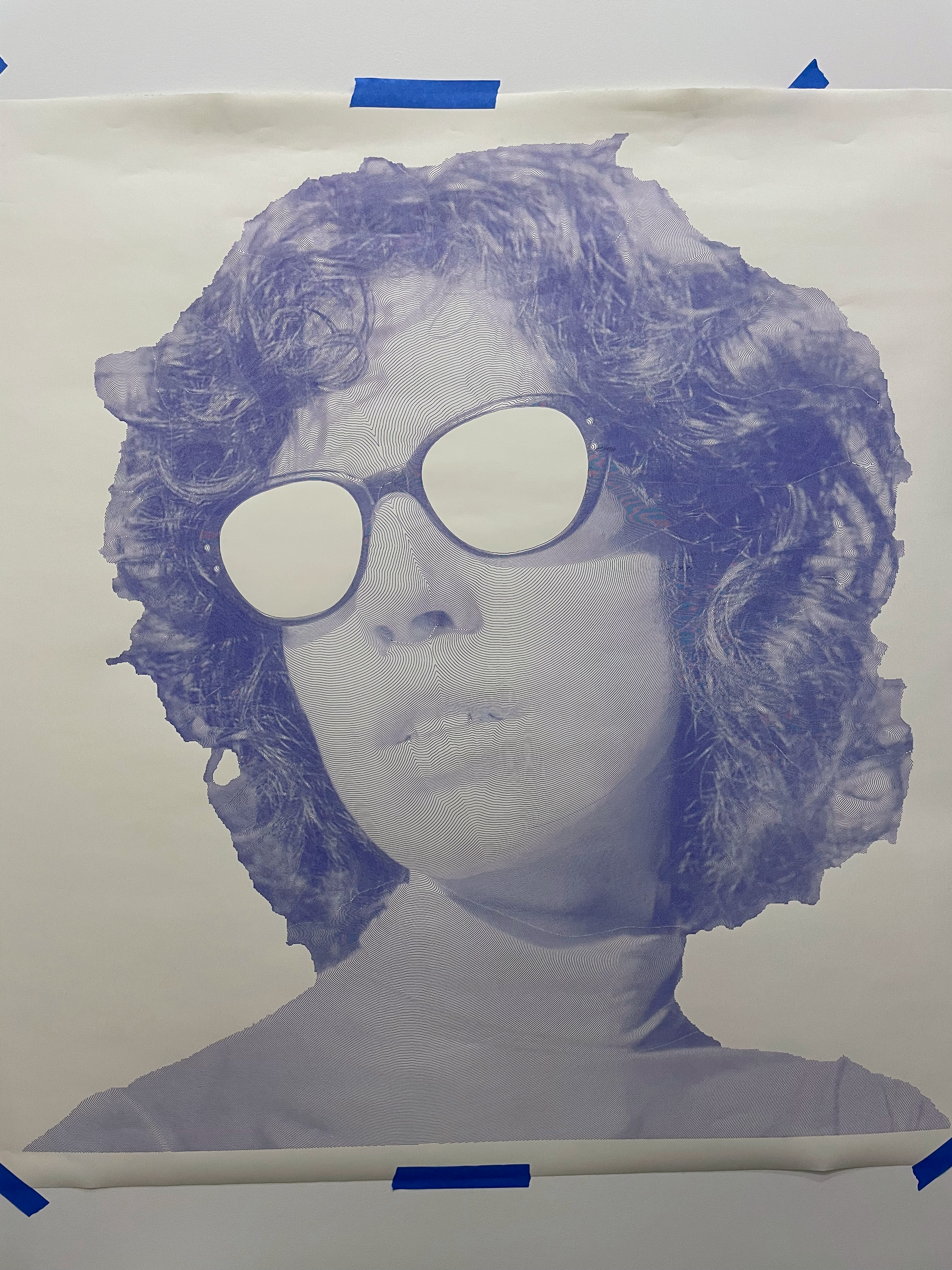
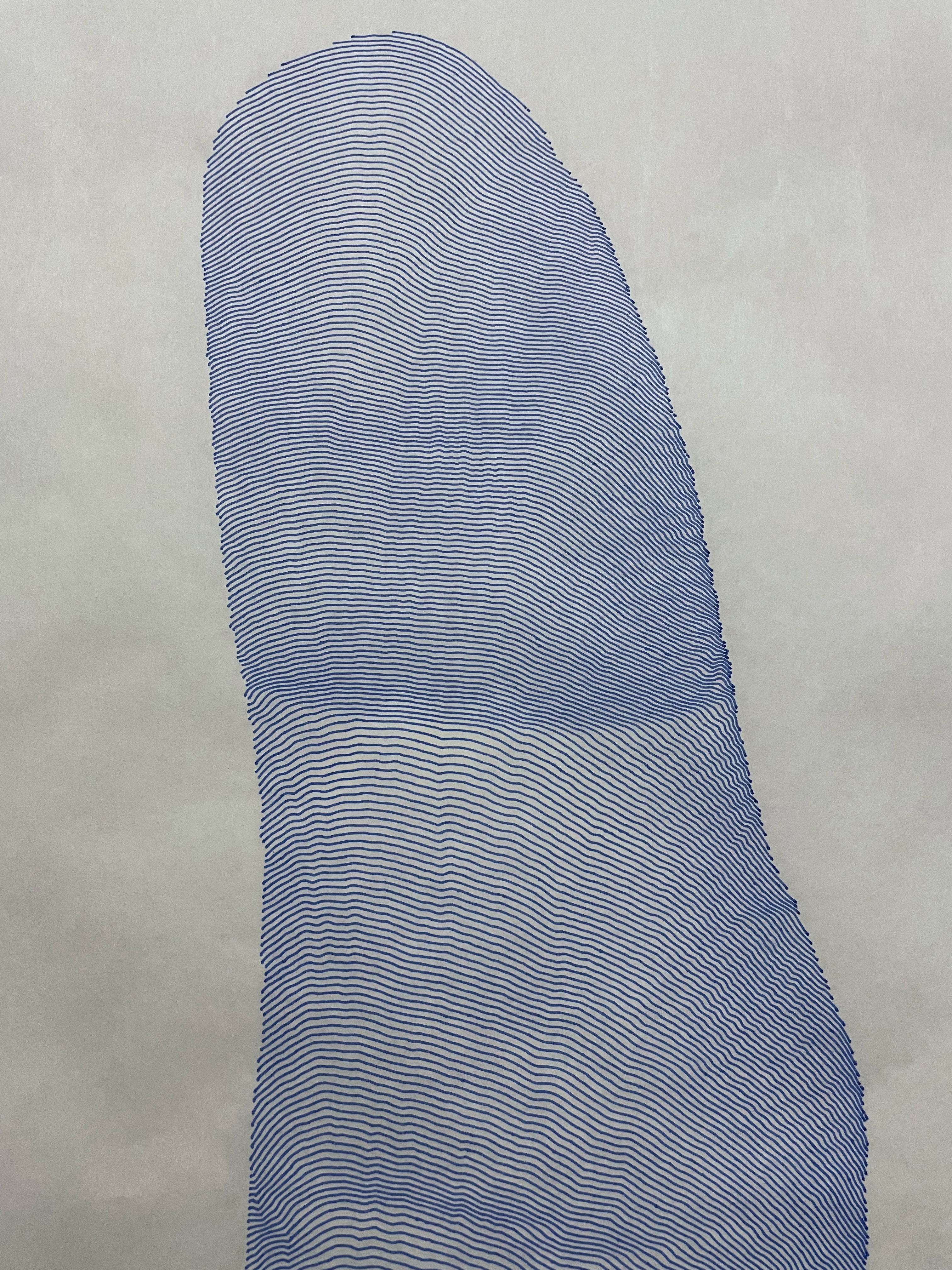
In January of 2018, I developed a new art style using gel pens, printer paper, and a lightbox for tracing. I printed out images in black and white, taped another piece of paper on top, shined a light through from underneath, and got to tracing. I made these:
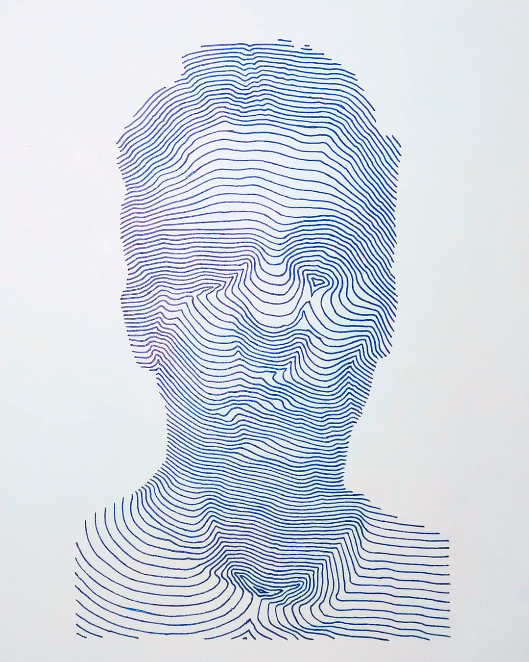
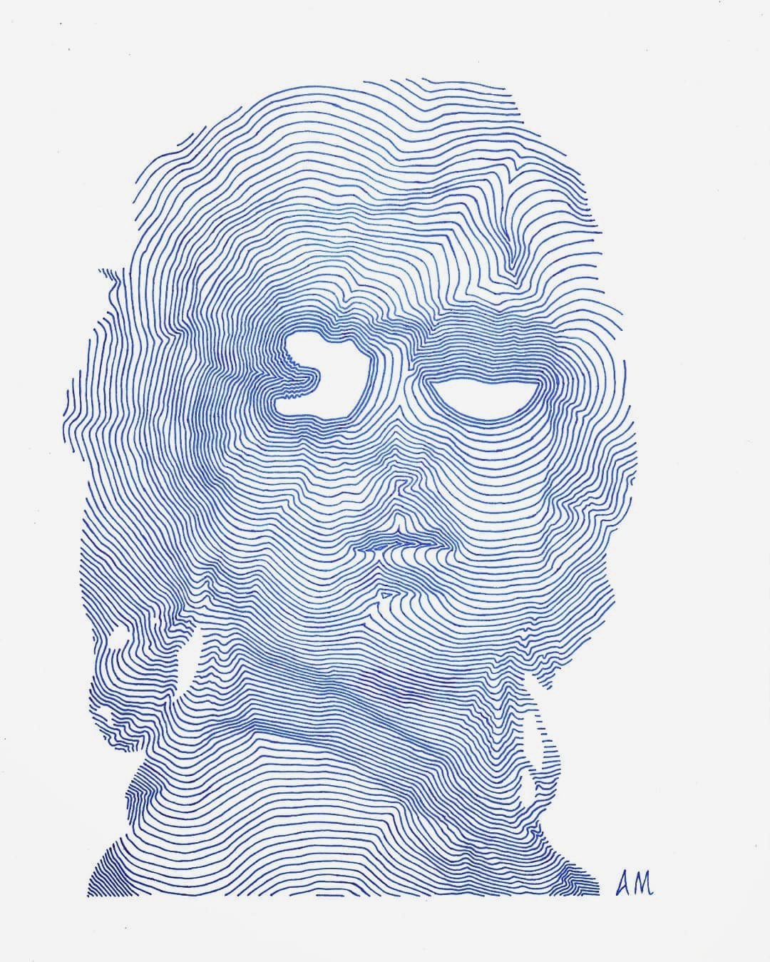
I still look to these pieces all the time for inspiration, but they were exhausting to make. Each took several hours to draw, hunched over a desk and slowly laying down one line at a time. I would certainly not be making anything larger than a standard sheet of paper using this method.
Going Digital
Later that year I started learning to code with Processing, a programming language made by and for artists. My work quickly focused on the art of image rendering, of filters and halftoning patterns, ways of reconstructing an image from a given set of geometric and chromatic constraints.
It wasn’t long before I started thinking about how to replicate my drawing style in Processing. If I could do that, I could use a pen plotter to make pieces as large and intricate as I like without having to draw them by hand. The prospect was exciting of course, but I also had the feeling that it would be impossible.
I started making attempts in late 2019, once I felt good enough at coding to give it a shot. I probably was, but my attempts went in the wrong direction. I tried to re-create the process too literally, making a virtual pen trace out each line. I’d been ignoring what was obvious to myself and many other people I had talked to — this style is a mathematical function.
The Math
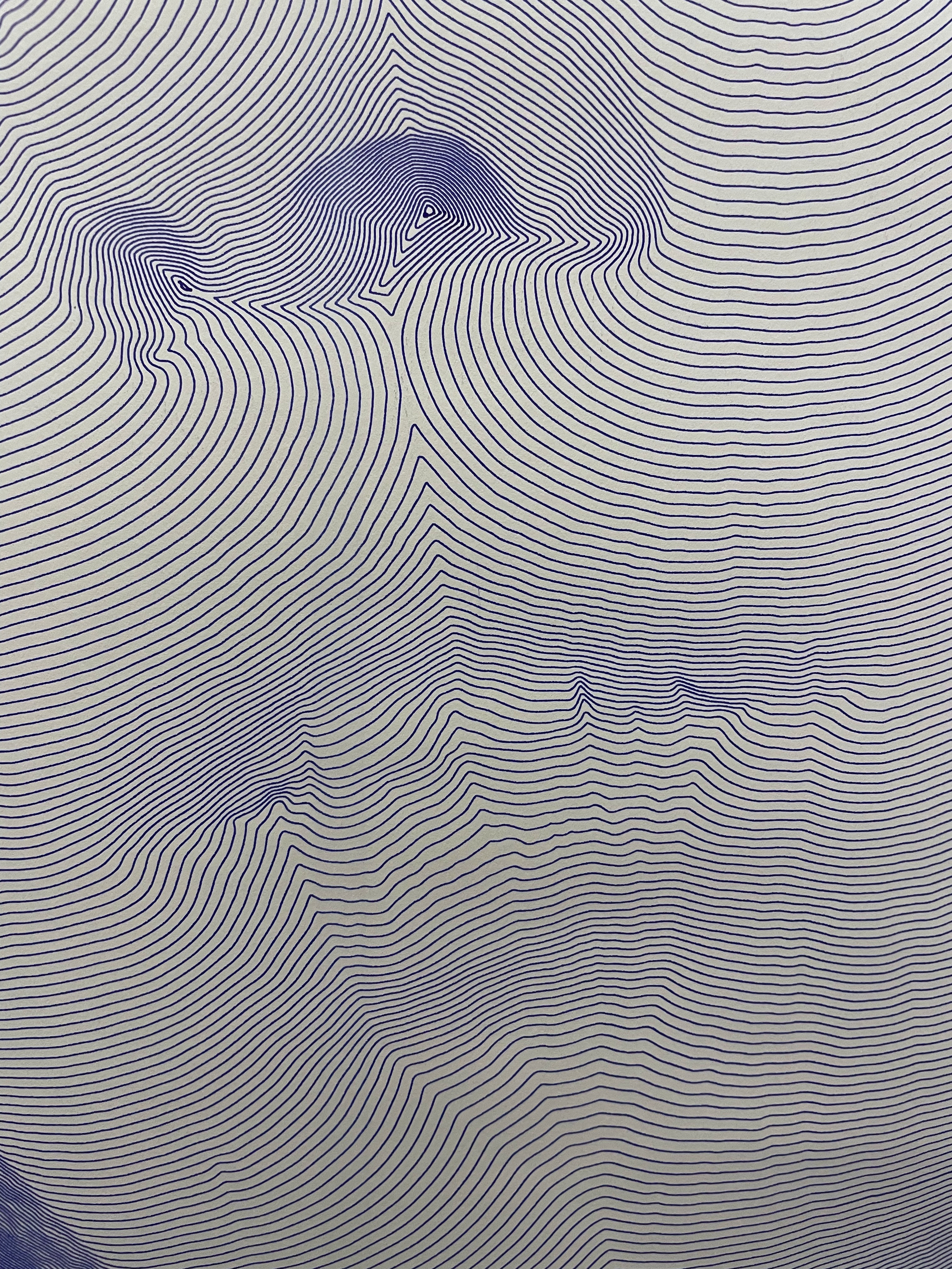
Someone fresh out of multivariable calculus might look at these drawings and write something like this:
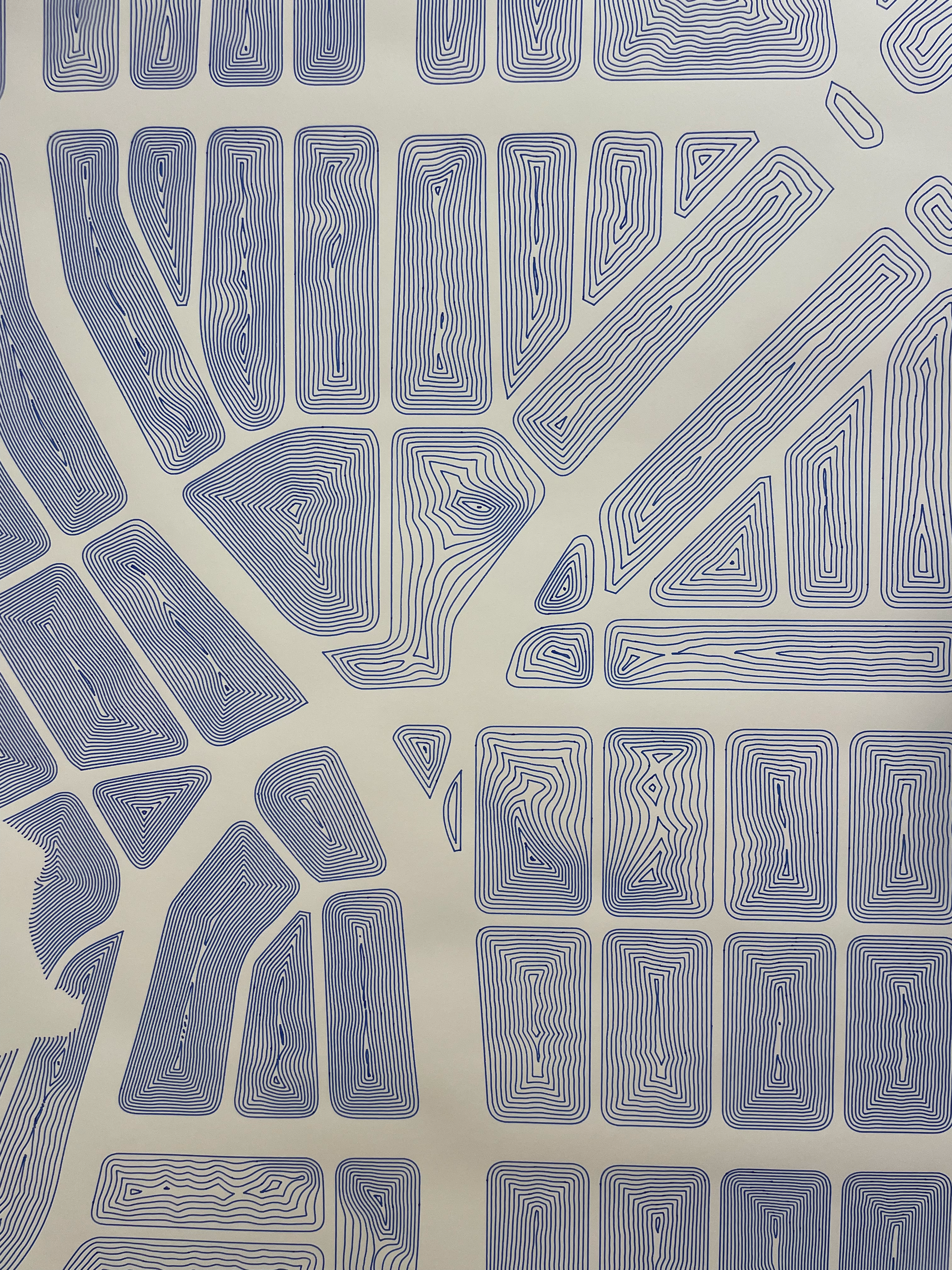
\[\|\nabla u(x,y)\| = f(x,y)\]If each drawing is a topographical map, $u(x,y)$ defines the terrain that’s being sliced to create it. The slices bunch up where the terrain is steepest, and spread out where it’s more shallow. This density is what creates the halftone effect, so the steepness of $u$’s surface must be controlled by the darkness of the desired image. We define the function $f(x,y)$ as that measured darkness, so in plain English our equation is:
“The slope of $u(x,y)$ at any given point $(x,y)$ is defined by the value of $f(x,y)$ at that point”
If you look back at the drawings, this equation can clearly be seen as the rule I was unknowingly following. The problem was solving it, and I had no ideas on how to even begin.
I got unstuck by pure chance in the Summer of 2020: I finally found the name of the equation I was trying to solve. I’ll admit that given how long it took me to stumble upon this name, and how crucial it was, it feels weird to just give it away. Anyway, it’s the Eikonal Equation.
The Algorithm
That Wikipedia article was the initial gateway to making my program, but there was a long road ahead — I was working right at the edge of my abilities as a mathematician and a programmer. Even writing out what the algorithm had to do, before any coding could begin, took the better part of a week. I’ll try to summarize it in a paragraph or two, but don’t get your hopes up.
Computers need to interpret smooth, continuous functions as measured points on a discrete grid (in this case, the pixel grid of the canvas). Rather than taking derivatives as we would on paper, they just directly measure the slope near a given point (which is just as well, because the Eikonal Equation has no closed-form solution anyway). We can sample the image at every pixel $(x,y)$ to get our $f(x,y)$ at each grid point, and assuming we know the (lowest) values $U_X ,U_Y$ of $u$ at the neighboring points in each direction, our equation can be written as:
\[\sqrt{\left(U_{ij} - U_X\right)^2 + \left(U_{ij} - U_Y\right)^2} = f_{ij}\]Where $U_{ij}$ is the value of $u$ at pixel $(i,j)$. We measure slope by subtracting the values of neighboring points, and then take the Euclidean norm to get $|\nabla u(x,y)|$. Feel free to grab a beer and spend an afternoon solving this; otherwise you’ll just have to trust me when I say that the solution is:
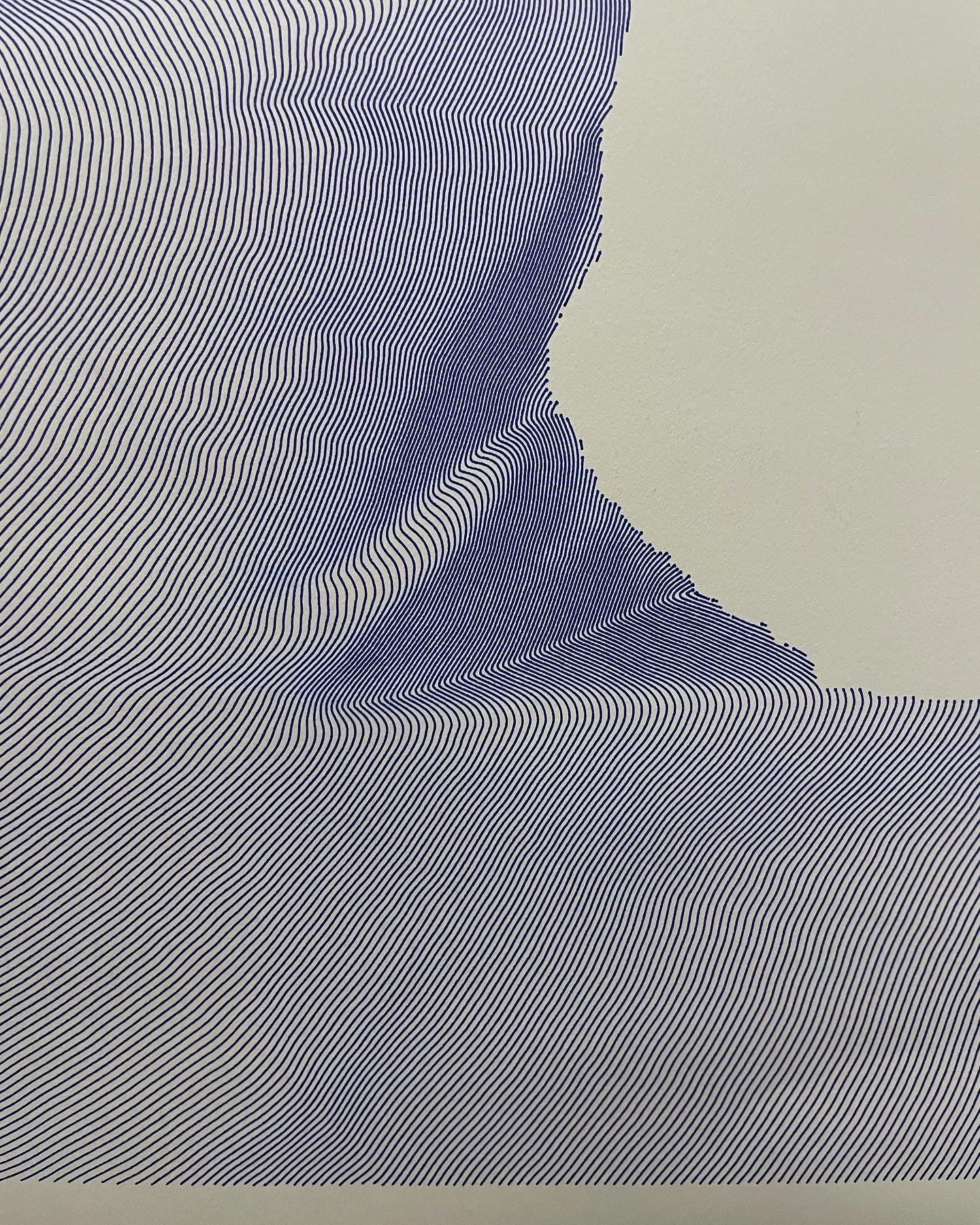
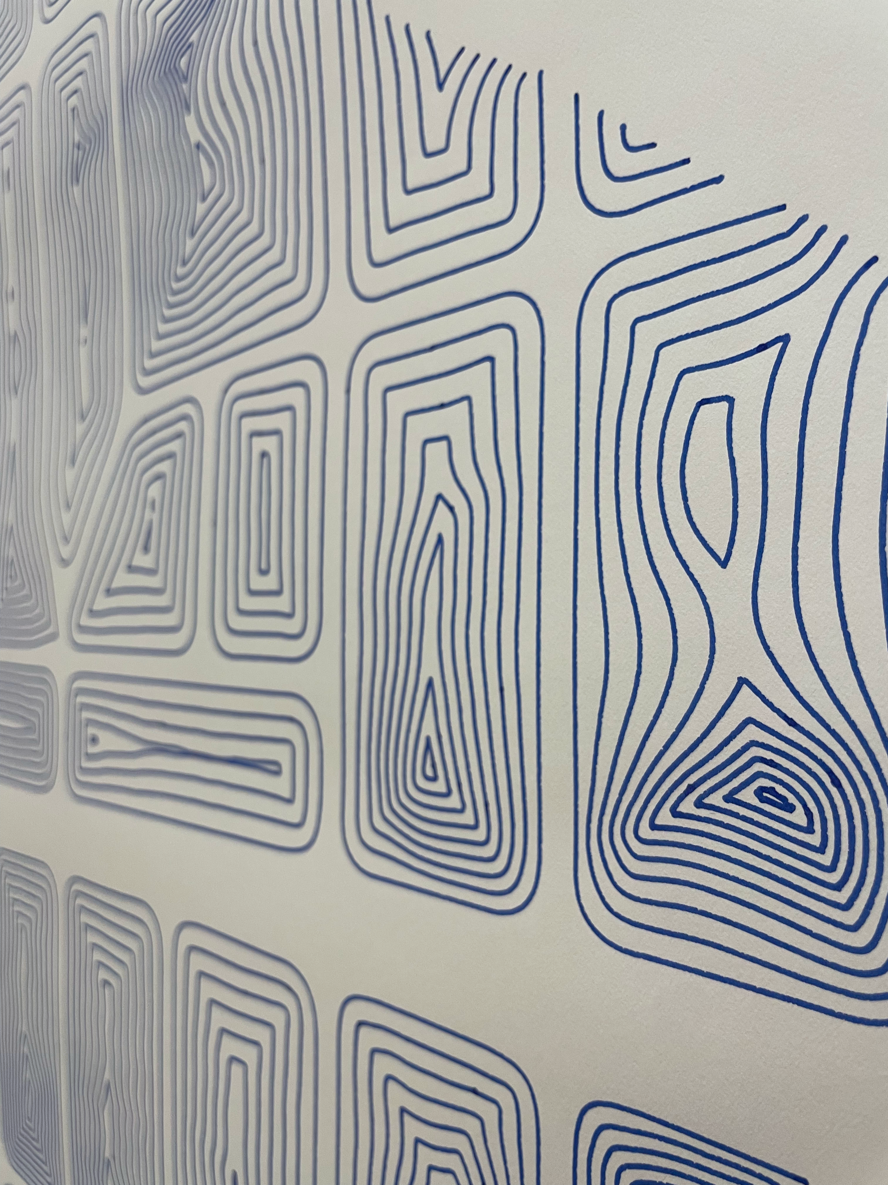
\[U_{ij} = \frac{U_X + U_Y}{2} + \frac{1}{2}\sqrt{\left(U_X+U_Y\right)^2 - 2 \left(U_X^2 + U_Y^2 - f_{ij}^2 \right)}\]Great! We have the closest thing to a closed-form solution. And it’s so pretty. Problem is, it relies on already knowing the value of $u$ for at least one neighboring point. This makes sense in a way — you can imagine the contour lines as waves rippling out across the canvas from one point or direction. Changes in their shape early on will affect the shape they take later. Since one part of the domain can have such an effect on the other, it becomes more clear why there is no closed-form solution. This long chain of cause-and effect is why there is no way to solve this equation everywhere all at once.
This is where James Sethian’s Fast Marching Method comes in. It’s an algorithm that takes a set of points with known values, which I call the origin, and builds the solution out from them one point at a time. If you’re familiar with Dijkstra’s Algorithm, you’ll be able to see the third interpretation of this equation’s solution: the path-distance of each point from the origin, where $f$ is affecting the speed of travel. You can see it in this old map:
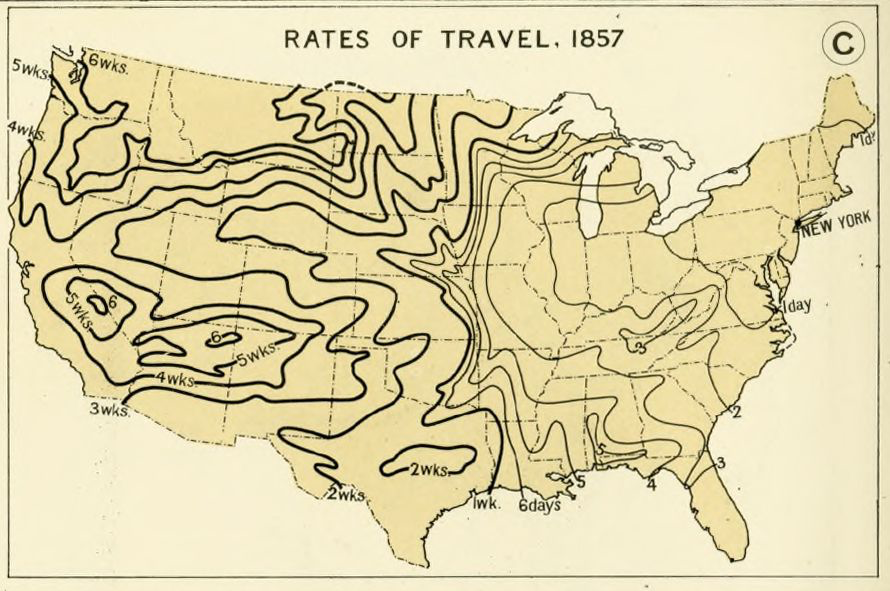
Fast Marching is basically Dijkstra’s Algorithm, using the expression from before as its method of measuring path-distance. And once we’ve implemented it, we can solve the equation! This is the very heart of the program (I only operate on it when something has gone horribly wrong). To make it usable, we need an interface with which to make and export designs.
The Interface
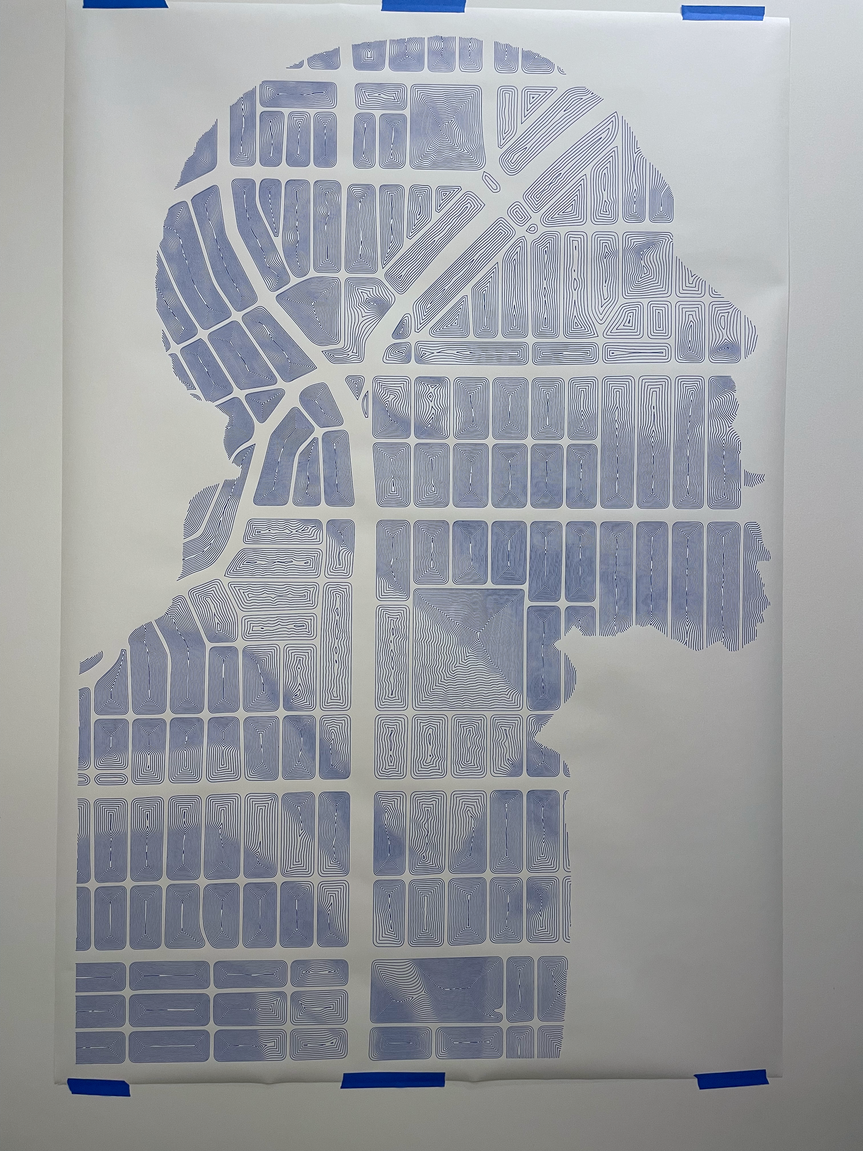
Making the interface I use to try out ideas and export designs has been a continous process. I tinker with it and add features whenever I need it to do something new, or when I’m not happy with the results. It’s changed a lot over the years, but here’s what it currently looks like:
Pre-processing happens in Photoshop. The background is masked out in blue, which tells the program what regions to ignore. The subject is in grayscale, and red gives the origin set — the pixels with a known solution (zero) from which the solution for the rest of the domain can be grown. The red can be drawn in the program to try out ideas quickly, or added during pre-processing for more precision.
Once the solution is complete, the contour lines can be exported as a vector file, ready for any cutting or drawing machine. I used Marching Squares to draw the contours, and a custom sorting algorithm to join all the tiny line segments into continous paths.
That part alone took as long as getting the thing working in the first place. But once it was completed, all I had to do was send finished designs to a pen plotter and watch it draw designs as big and detailed as I wanted. Finally, I thought, now comes the easy part.
Manufacturing
Everything described thus far took about 5% as long as it took to actually develop the manufacturing process.
Once I had the program working, I tried and failed to get good results from my cheap desktop plotter. With no other resources at my disposal, I gave up on this project for the time being. When UCLA resumed in-person classes a year later, I started my favorite job again: working at the residential makerspace. Somewhere in the middle of Fall quarter, I realized that our huge vinyl cutter was the perfect machine to make the art pieces I had been dreaming of. And so, from October 2021 to May 2022, I spent every weekend and most weekdays hunched over our Roland GR-420 vinyl cutter.
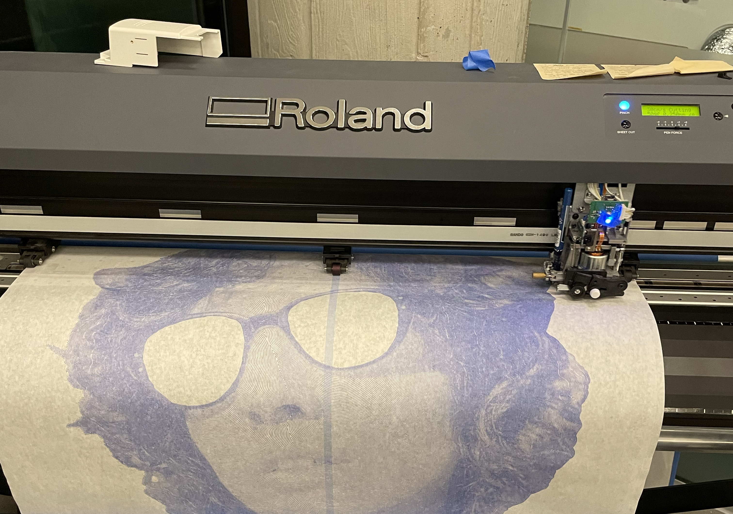
Normally this machine takes rolls of vinyl up to 42 inches wide and cuts them with a drag knife. Replace vinyl with paper and knife with pen, and you have a giant plotter. It was not only much larger, but much more precise than the one I had at home. On more detailed pieces, a line being off by even a tenth of a millimeter can cause visible banding. This machine would draw all across the paper for hours, laying down literal miles of lines, and never drift by even that much. For its intended purpose it had no reason to be capable of doing this, but it was.
When I started working with the Roland, I would’ve been appalled at the idea of writing this article — I had long been afraid of other people stealing my source code and replicating my pieces. Seven months of work later, I was no longer worried. The additional knowledge required to get the results I want on paper exists only in my head, and I acquired it by going far past the point where any sane person would’ve given up.
With no existing reference available, I had to push through very specific and unprecedented problems with ink flow, smearing, paper movement, acceleration curves, anti-aliasing… the list goes on. At the moment, the only way to find the solutions to them is through months of trial-and-error. Those are the secrets I will keep for now.
The technique has progressed only in small ways since then. In March 2023 I discovered a fundamental math error while writing the first draft of this article. I did some heart surgery on the program and saw a significant difference in the resulting patterns. I’m not sure if I like it more. We’ll have to see.
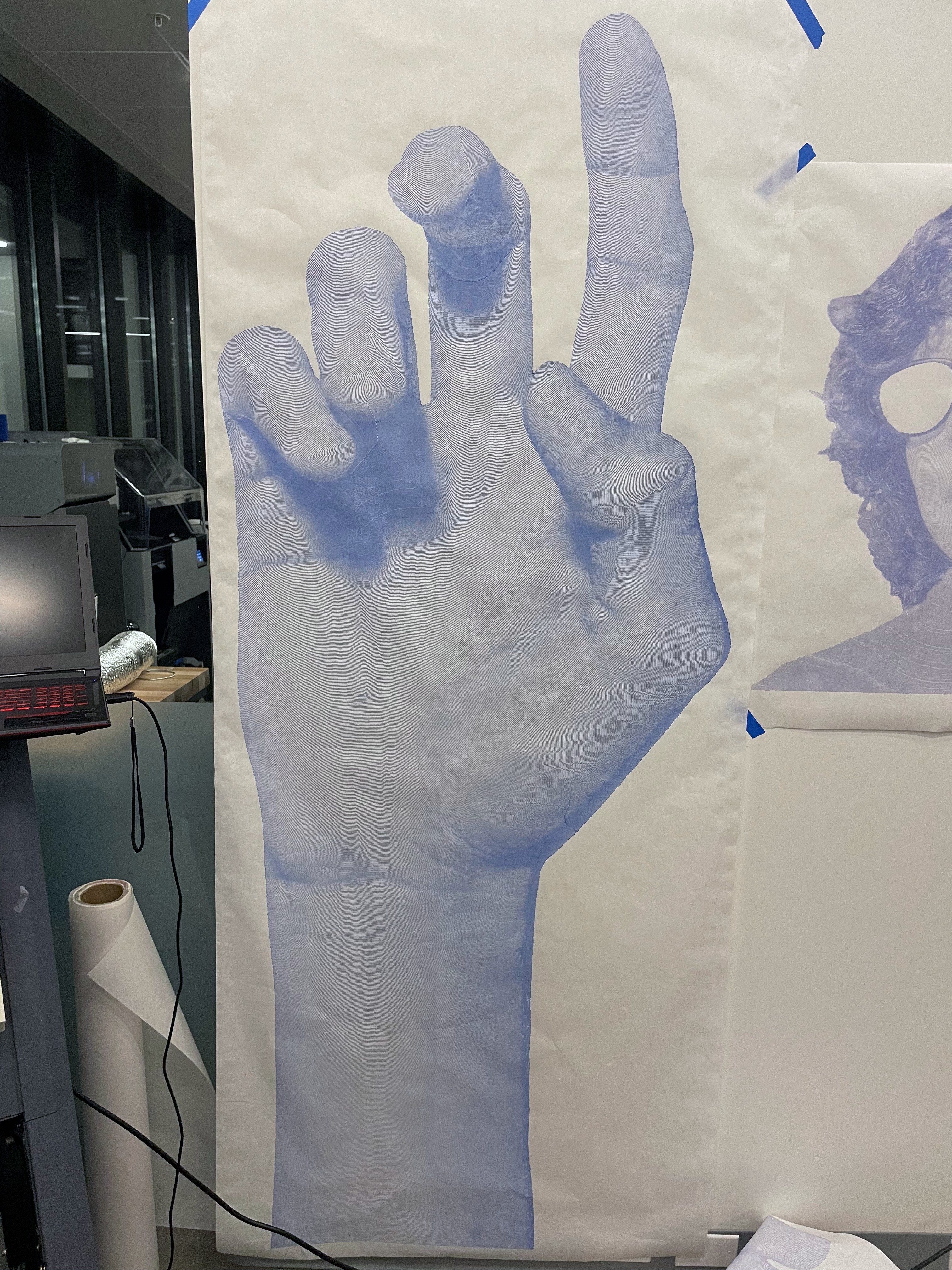
Gallery
Here are some of the pieces I made in 2021 and 2022: